
Positioning our portfolio so that it’s optimised for the market environment
- Nick Bird
- Jul 28, 2023
- 7 min read
Updated: Sep 28, 2023
The most distinctive feature of our investment process is our non-systematic overlay.
Previously we’ve documented how we manually review stocks which satisfy our systematic stocks screens. We refer to this process as our “micro” non-systematic overlay.
In this research note, we document how we adjust portfolio positioning so that it’s best suited to the current market environment. We refer to this process as our “macro” non-systematic overlay.
The macro non-systematic overlay is facilitated by our LiDAR system. In broad terms, this system tells us how the current market environment looks vis-a-via our investment process.
System outputs include:
Factor performance data based on a range of metrics (eg rank ICs, naïve and pure factor returns),
Valuation spreads based on relative book yields,
Alpha factor correlations,
A/H relative performance (for Chinese equities),
Ex post beta analysis.
Based on interpretation of these outputs, the macro overlay is used for:
Factor timing
Country positioning
Identifying market specific risk factors
Determining the most appropriate short portfolio composition (futures versus stocks)
Adjusting portfolio gross exposure.
The implementation of our macro overlay is best illustrated by way of example. As much as possible, we have used topical examples so that they’re easily relatable.
Before going through the examples, we want to emphasise a key point: none of these macro overlays will dominate fund performance. The primary performance driver will always be our stock selection process. They are intended to be alpha accretive, with a focus on reducing downside volatility (which has been extremely low since we launched the fund).
Factor timing
We adjust alpha factor exposures based on our analysis of LiDAR outputs. We’ve looked at many factor timing quant models but there aren’t any which we believe are sufficiently robust to include in our systematic investment process.
The main problem with these models is lack of breadth. With limited breadth, you need strong backtest results to improve risk adjusted performance. Also, quant models with limited breadth (or degrees of freedom) are prone to data mining. For example, if you tweak a factor timing model so that you increase exposure to value factors from 2001 to 2007 and growth factors from 2015 to 2020, you’ll get great results. However, the model is more likely to be the product of a data mining exercise rather than anything substantive that will work in real life (ie out-of-sample).
However, we believe that if you have a trained eye analysing the relevant data, particularly if that data is displayed in a user-friendly way and you understand how that data relates to the current market environment, you can make informed decisions which can generate alpha.
Consider the following real-life examples.
Example 1: Reducing weight to auto-correlation momentum factors
In 2020, auto-correlation momentum factors (exploiting the tendency for outperforming stocks to continue outperforming and vice versa) looked crowded. There is typically a negative correlation between these momentum factors and valuation factors. This is intuitive: outperforming stocks tend to be expensive and underperforming stocks tend to be cheap. However, in the second half of 2020 and the first half of the following year, the negative correlation was extreme. Further, the valuation spreads for the top and bottom quintile of stocks ranked by total returns over the last 1 to 2 years were extremely wide relative to historic averages. Outperforming stocks were incredibly expensive, and, in a relative sense, underperforming stocks were incredibly cheap.
Our reduced weight to momentum factors helped a lot in November 2020. Many quant factor funds performed extremely poorly that month, particularly in the first couple of weeks of November. The following links provide more information:
https://www.bloomberg.com/news/articles/2020-11-13/quant-shock-that-never-could-happen-hits-wall-street-models#xj4y7vzkg https://www.intalcon.com/magazine/the-11-9-quant-crash
Our fund performed relatively well in November 2020, registering a gross return slightly better than -1%.
It’s also worth noting that this positioning hurt fund performance in the months leading up to November 2020 and in several subsequent months. We’re ok with this given we’re happy to sacrifice some upside if we can mitigate downside risks.
Example 2: Increasing weight to value factors
We had an outsized value bias from when the fund was launched up until early 2022. This was primarily because, no matter how we sliced and diced the data, valuation spreads were extreme, even wider than during the peak of the tech bubble in the early 2000s.
The following link provides more detail on this topic, including numerous charts extracted from LiDAR: https://www.oqfundsmanagement.com/post/extreme-value-spreads-in-asia.
It’s worth noting that our net value exposure wasn’t so extreme that we couldn’t generate strong returns when value factors underperformed. Indeed, the fund performed well from 2020 to the end of 2021 when value factors got crushed.
Country positioning
As we’ve previously documented, we will take informed risk “tilts” when we think they’ll be alpha accretive. The alternative – ie maintaining really tight risk exposures – requires high leverage to generate decent return volatility (and hence decent headline returns). This is normally ok, but during market dislocations can result in forced unwinding and extreme losses (witness what occurred to many quant factor funds in August 2007). Another potential source of return volatility – concentrated stock bets – isn’t compatible with our style of investing.
Example: Net China exposure
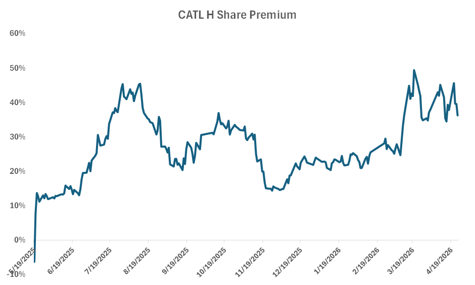
In many ways, Chinese equities are interesting. There are the ‘A’ shares listed in Shanghai and Shenzhen, the ‘H’ shares listed in Hong Kong, and numerous Chinese ADRs listed in the United States. Many companies are dual listed in China and HK (ie have ‘A’ and ‘H’ shares). These shares aren’t fungible and hence they trade at either a premium or discount based on liquidity flows.
In the second half of 2020, and most of the following 2 years, ‘A’ shares were trading at a significant premium to their ‘H’ share counterparts. There were several instances when the ‘A’ share of every dual listed stock traded at a premium to its ‘H’ share counterpart (and as at the time of writing, 28 July, this is also the case). In many cases this premium has been (and still is) extremely large. For example, some large and liquid ‘A’ shares trade at more than three times the currency adjusted ‘H’ share price. It should be noted that ‘H’ shares have the same voting and dividend rights (and hence many ‘H’ shares have a much higher dividend yield than their ‘A’ share counterparts).
Also, during 2020 and much of 2021, there were many Chinese ADR shares which were only listed in the United States which rated relatively poorly based on our stock selection process.
Given this, our Chinese equities “risk bucket” included a net short exposure to ‘A’ shares (mainly through China A50 futures contracts listed in HK and Singapore), a net short exposure to Chinese ADRs, and a net long exposure to ‘H’ shares listed in HK. As a side issue, this is one of the many issues which potentially adversely impact how vendors do their idiosyncratic risk analysis. They looks at “country of listing” rather than “country of risk”. We believe the second approach is superior.
Finally, the Hong Kong market is interesting in that there are several large stocks which primarily have European and global exposure (eg Prada, CK Hutchison, Samsonite, L’Occitane, NagaCorp). When Chinese equities are getting sold off aggressively, these stocks tend to fall in line with the overall market despite their lack of direct Chinese exposure. We do not categorise these stocks in our China risk grouping.
Short exposure composition (futures versus stocks)
The biggest risk factor is clearly market beta. To maintain market neutrality, we need to offset our long stock exposure with a market beta equivalent short portfolio. This portfolio comprises stock and index futures positions (we don’t have any options in the portfolio).
Example: Getting more short exposure via index futures
The second half of 2020 and the first half of 2021 were characterised by excess liquidity fuelled by highly accommodative monetary and fiscal policies. There was too much money chasing too few investment opportunities. This was epitomized by the meme stock mania (eg GameStop, Carvana).
In this environment it’s difficult and potentially very dangerous shorting stocks (witness the demise to Melvin Capital).
To deal with this, we got significantly more short exposure from index futures than normal. In 2021, our short exposure from futures peaked at close to 50% (see chart below).
Chart 1: Futures percentage relative to total short portfolio

Source: OQFM
This wasn’t ideal as index futures are only a risk mitigation tool rather than a source of alpha. However, we believe it was prudent given the level of investor euphoria and the extreme liquidity driven price distortions.
Market specific risk factors
We don’t like optimisers and risk models calibrated based on historic data. Optimisers are opaque and, given markets are fluid, risk factors emerge which are specific to the current market environment. Some of these risk factors are too ephemeral to warrant any corrective action. Others affect market sentiment, but their impact is muted. Our primary concern is risk factors (not included in risk models) which are having a big impact on investor sentiment and where the impact is likely to continue for a prolonged period.
Example: Controlling for Covid risks
Covid was a once in a 100-year pandemic and Covid risk wasn’t captured by models calibrated using historic data. We adjusted for Covid as a risk factor when the fund was launched, in the knowledge that various scientists were working on vaccines, and the share prices of Covid impacted stocks could move dramatically based on any vaccine developments. This helped mitigate losses during the turning point that occurred when mRNA vaccine efficacy results were released.
Reducing gross exposure
Typically, we set gross exposure at a level commensurate with our fund return volatility target (7% pa based on daily gross performance data). As a result, we reduce gross exposure when market cross-sectional volatility is high and vice versa.
When the market environment isn’t conducive to our style of investing, we will endeavour to reposition the portfolio so that we can still generate alpha. The aforementioned examples illustrate this. However, during exceptional market environments when we can’t think of a good way of doing this, we will reduce gross exposure.
Example: Great Recession of 2008
These events are rare, so we need to go back a long way to find a good example. In the second half of 2008, all sorts of market dislocations were taking place. Analysts didn’t know how to react to the changing market environment and their forecasts were stale. This impacted the veracity of the data feeding into numerous quant factors, particularly valuation and sentiment factors. We responded by using value factors based on historic normalized data (rather than analyst forecasts data), but this wasn’t a panacea.
The ultimate defense was to “take money off the table”. We cut gross exposure in the second half of 2008 to deal with the extreme market environment and limit any potential drawdown.


Comments